A hands on introduction to Engineering Simulations

Table of Contents

What Does Simulation Actually Mean?

Say you’re designing a bridge, a turbine blade, or even just a heated pan. You want to know: Will it bend under weight? How fast will fluid flow past it? How hot will it get?

Instead of building dozens of prototypes and measuring things physically, we simulate them. But how do we do that?

That’s where methods like Finite Element Analysis (FEA), Finite Volume Method (FVM), and Computational Fluid Dynamics (CFD) come into play. These aren’t magic tools—they use numerical methods to convert real-world physical equations into results on a computer screen.

But before we get into all that, let’s rewind and start with a concept that unites them all:

Discretization

Imagine we’re trying to find out how heat spreads across a metal plate. The metal plate becomes our domain.

Mathematically, this is governed by the heat conduction equation, a differential equation that says: “temperature depends on how much heat is flowing in or out of every point in the material.”

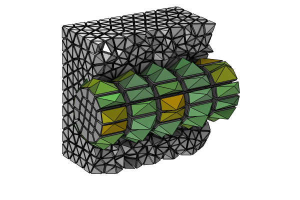
But a computer can’t solve something that’s defined at every possible point (which are infinite!). So we divide the entire domain into smaller subregions. These could be triangles, rectangles, tetrahedrons, etc.

These small pieces are called elements (in FEA) or cells (in FVM). The process is called meshing.

At the corners & centers of these regions, we define nodes & cell centers respectively. These are the discrete points where we will calculate our primary physical variables:

Temperature (in heat transfer problems)
Displacement in x/y/z (in structural problems)
Velocity and pressure (in fluid problems)

Meshing a structure means splitting it into tiny manageable regions with nodes/cells.

Once we know values at these discrete locations, we use interpolation to fill in the rest of the space in between. That’s how simulation results become colorful contour plots.

Why Just at the Nodes or Cell Centers?

Each node is a “sampling point.” Trying to store the value at every location in a solid or fluid would be impossible—so we just calculate it at certain locations. The equations are formulated such that they describe what’s happening around that node based on the surrounding conditions.

Instead of solving an equation for every molecule in a pipe, we pick a grid of important locations and solve them there.

The smaller the cells, the more nodes, the more accurate—but the more expensive (computationally) the simulation becomes. And the harder it gets for the solution to converge.

To get a more accurate solution, we can either increase the number of cells(using a finer mesh), or we can increase the number of nodes.

Local & Global Conservation

Let’s say we’re simulating fluid flowing into a pipe. We expect whatever goes in to eventually come out. This is called conservation of mass. If our simulation somehow shows that more mass comes out than goes in, something is seriously wrong.

This is where a fundamental difference between FEM and FVM comes in.

In FEM, we write our equations in a way that solves for variables at nodes. But conservation (like energy or mass) isn’t automatically guaranteed in each small element. It’s only ensured overall, across the entire domain. This is global conservation.

In FVM, we apply our physical laws directly over each control volume (cell). That means each small cell conserves mass, momentum, and energy independently. This is called local conservation.

That’s why FVM is preferred for fluid flow problems - which are very sensitive to any non-conservation.

What Are We Actually Solving?

Let’s take a few different physical scenarios and peel back what’s going on.

🔥 Case 1: Heat Transfer (Thermal)

If we heat one end of a rod, the heat flows to the other end. This is governed by Fourier’s Law:

$$ q = -k \nabla T $$

It says that heat flux is proportional to the negative gradient of temperature.

This gives us a differential equation:

$$ \frac{\partial^2 T}{\partial x^2} + \frac{\partial^2 T}{\partial y^2} = 0 $$

Now, to solve this on a computer, we approximate this differential equation into a set of equations that can be solved algebraically.

In FEM, this is done using an approach called the weighted residual method, where we multiply the differential equation with a trial function and integrate over the domain. This converts the equation into what we call the weak form—don’t worry too much about the name.

The end result looks like this:

$$ [K] \{T\} = \{Q\} $$

Where:

$[K]$ is the global conductivity matrix
${T}$ is the vector of temperatures at each node
${Q}$ is the vector of heat inputs or boundary conditions

We solve this system using techniques like matrix inversion, which gives us the temperatures at each node. Then interpolate to get the temperatures throughout the domain. The other effects, like heat flow, heat flux, etc., can be derived from these nodal temperatures. This is called post-processing.

🧱 Case 2: Structural Mechanics

Imagine a beam under load.

Each node can move in x, y, z directions → 3 unknowns per node. The computer solves a system of 3x equations for x nodes. Some nodes are fixed. Others might experience force.

The governing law is Newton’s second law—force = mass × acceleration, which simplifies to just force balance in static problems.

The final system of equations again looks like:

$$ [K] \{u\} = \{F\} $$

Where:

$[K]$: Stiffness matrix
${u}$: Displacement vector
${F}$: External force vector

Solving this gives us the displacement of each node in each direction. Then using basic stress-strain laws (Hooke’s law), we calculate stresses and strains- which is again post-processing.

🌊 Case 3: Fluid Flow (CFD)

Fluids are governed by a set of equations called the Navier-Stokes equations, which enforce conservation of mass, momentum, and energy.

In FVM, we don’t work with point-based differential equations. Instead, we work with integral forms of these laws over small control volumes (cells).

The general form is:

$$ \frac{\partial}{\partial t} \int_V \phi \, dV + \int_A \phi \vec{v} \cdot d\vec{A} = \int_V S_\phi \, dV $$

The problem is, these equations are non-linear, meaning their solutions are not straight lines or simple curves.

We start with a guess. The solver uses methods like Newton-Raphson to refine the guess.

Newton-Raphson Method

Imagine you’re trying to find where a curve crosses the x-axis. You pick a point on the curve. Draw a tangent. Your next guess is where that tangent cuts the x-axis. Repeat this process.

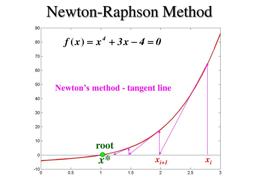
That’s Newton-Raphson. It’s a method to iteratively approach the solution to a non-linear equation by drawing successive tangents.

Each iteration gets us closer to the right answer.

This process continues until the difference between two guesses (called the residual) is very small. If this residual is large and keeps growing, our simulation is diverging. If the residual becomes very small and stays low(usually less than $ 1 \times 10^{-6} $), our simulation is converging.

So in CFD, we often monitor the residuals to check how good the solution is getting.

Direct Numerical Simulation (DNS)

There’s actually another way to solve fluid problems, called the Direct Numerical Simulation (DNS). Here, we solve the Navier-Stokes equations exactly— capturing every tiny swirl and vortex in the flow.

Although it sounds perfect, it is computationally the most challenging, often requiring billions of grid points even for simple flows. Due to the high computational cost, it has been mostly limited to academic research & high end supercomputers.

With the advent of GPUs & Fluidx3D, a promising future lies ahead.

Simulation Workflow

We’ve split our domain, selected our physics, and written down some equations. But how does this whole thing come together?

1. Pre-analysis

Before even opening a simulation software, we take a pause and examine what’s really happening in our system.

Is it thermal, structural, fluid-related or something more?

Can it be simplified to 2D?

Is it steady (doesn’t change with time) or unsteady?

Are there any obvious symmetries we can exploit?

This is where we sketch free-body diagrams, write down governing equations, and do a few hand calculations to get an estimate of the result.

For example: “If 1000 N force is applied on this beam, we can expect a deflection of around 1 mm. Let’s see what the simulation says.”

2. Geometry and Meshing

Once the problem is understood, we can bring in the geometry— either manually drawn or imported from CAD. Remove small holes or text embossings that don’t affect physics. Split the domain into elements (FEM) or cells (FVM).

This is meshing—and it’s one of the most important steps. It’s where we choose how finely to chop up our domain.

Finer mesh → more accuracy → longer solve time.

Coarser mesh → faster → may miss critical behavior.

Mesh too fine, and our simulation might take days to compute, without an appreciable change in solution accuracy. Too coarse, and we might not capture boundary conditions, flow separation and other essential behaviour properly.

3. Boundary Conditions

This is where we specify where the system is fixed, which forces are applied, which temperatures are known, and where the fluid enters and leaves.

No simulation can run without boundary conditions. They define how the system interacts with the outside world.

For thermal: Fix the temperature on one side, allow convection on another.

For structural: Fix a support, and apply a force.

For fluids: Define the inlet velocity or pressure, and specify an outlet.

This step defines the problem. Our equations are incomplete without boundary conditions.

4. Solve

Now comes the heavy lifting. The solver translates our discretized domain and governing equations into a massive system of algebraic equations.

In FEA, it assembles matrices and directly solves them.

In CFD it begins with a guessed solution, then iteratively corrects it, usually through something like Newton-Raphson.

If the solution diverges, our mesh might be too coarse, or the boundary conditions might be off. We will look at how to fix this in upcoming posts.

We start with a coarse mesh, get an approximate solution, then refine it iteratively to get to a better solution, until an appreciable change in the solution is not obtained. This is known as mesh refinement.

5. Post-processing

Once solved, we now have the numbers at the nodes or cell centers. But that’s not what we’re interested in. We want to know:

Where is it hottest?

How much did it deform?

How fast is the fluid going there?

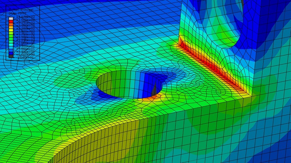
We use interpolation to derive all other results and fill in values between the points(nodes/cells) and display them using contours, arrows, and 3D plots.

This is how the beautiful rainbow plots are born.

6. Verification

We try to analyse if we’ve solved the math correctly. Does the result match known analytical solutions?

Do total forces balance?

Are mass and energy conserved?

We also use hand calculations with minor simplifications to predict the expected results. If results are entirely different, we need to go back to Step 1 and try again.

7. Validation

We compare the simulation to experimental data.

If simulation says 102°C and real-world sensor reads 98°C— we’re ~4% off. That’s a validation gap. Validating with real world data is the fundamental check that shows how much our simulation is off.

Verification and Validation are the most crucial steps in simulations, since they help us validate our results. A computer might spit out garbage, but its upto us to make sense of it.

Simulations Aren’t Just Button-Pushing

Many users treat simulation software as magic boxes:

Import geometry → Click solve → Export pretty image.

But without understanding what’s happening behind the scenes, you could be getting entirely wrong answers—and not even know it.

Understanding why we split the domain, what we solve at each point, and how governing equations are transformed gives you the power to spot bad results, refine mesh only where needed & validate with confidence.